Creating and modelling metallic supercells
![]()
![]()
In this section we will be concerned with modelling supercells of aluminium. When dealing with periodic problems there is no unique definition of the lattice: Clearly any duplication of the lattice along an axis is also a valid repetitive unit to describe exactly the same system. This is exactly what a supercell is: An $n$-fold repetition along one of the axes of the original lattice.
The following code achieves this for aluminium:
using DFTK
using LinearAlgebra
using ASEconvert

function aluminium_setup(repeat=1; Ecut=7.0, kgrid=[2, 2, 2])
    a = 7.65339
    lattice = a * Matrix(I, 3, 3)
    Al = ElementPsp(:Al; psp=load_psp("hgh/lda/al-q3"))
    atoms     = [Al, Al, Al, Al]
    positions = [[0.0, 0.0, 0.0], [0.0, 0.5, 0.5], [0.5, 0.0, 0.5], [0.5, 0.5, 0.0]]
    unit_cell = periodic_system(lattice, atoms, positions)

    # Make supercell in ASE:
    # We convert our lattice to the conventions used in ASE, make the supercell
    # and then convert back ...
    supercell_ase = convert_ase(unit_cell) * pytuple((repeat, 1, 1))
    supercell     = pyconvert(AbstractSystem, supercell_ase)

    # Unfortunately right now the conversion to ASE drops the pseudopotential information,
    # so we need to reattach it:
    supercell = attach_psp(supercell; Al="hgh/lda/al-q3")

    # Construct an LDA model and discretise
    # Note: We disable symmetries explicitly here. Otherwise the problem sizes
    #       we are able to run on the CI are too simple to observe the numerical
    #       instabilities we want to trigger here.
    model = model_LDA(supercell; temperature=1e-3, symmetries=false)
    PlaneWaveBasis(model; Ecut, kgrid)
end;
As part of the code we are using a routine inside the ASE, the atomistic simulation environment for creating the supercell and make use of the two-way interoperability of DFTK and ASE. For more details on this aspect see the documentation on Input and output formats.
Write an example supercell structure to a file to plot it:
setup = aluminium_setup(5)
convert_ase(periodic_system(setup.model)).write("al_supercell.png")
Python: None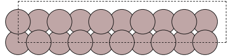
As we will see in this notebook the modelling of a system generally becomes harder if the system becomes larger.
- This sounds like a trivial statement as per se the cost per SCF step increases as the system (and thus $N$) gets larger.
- But there is more to it: If one is not careful also the number of SCF iterations increases as the system gets larger.
- The aim of a proper computational treatment of such supercells is therefore to ensure that the number of SCF iterations remains constant when the system size increases.
For achieving the latter DFTK by default employs the LdosMixing preconditioner [HL2021] during the SCF iterations. This mixing approach is completely parameter free, but still automatically adapts to the treated system in order to efficiently prevent charge sloshing. As a result, modelling aluminium slabs indeed takes roughly the same number of SCF iterations irrespective of the supercell size:
M. F. Herbst and A. Levitt. Black-box inhomogeneous preconditioning for self-consistent field iterations in density functional theory. J. Phys. Cond. Matt 33 085503 (2021). ArXiv:2009.01665
self_consistent_field(aluminium_setup(1); tol=1e-4);┌ Warning: Skipping atomic property pseudopotential, which is not supported in ASE.
└ @ ASEconvert ~/.julia/packages/ASEconvert/yMJC2/src/ase_conversions.jl:100
n Energy log10(ΔE) log10(Δρ) Diag Δtime
--- --------------- --------- --------- ---- ------
1 -8.298653767253 -0.85 5.0 151ms
2 -8.300234774744 -2.80 -1.26 1.0 98.9ms
3 -8.300442001037 -3.68 -1.90 2.9 99.1ms
4 -8.300461307504 -4.71 -2.78 1.1 76.8ms
5 -8.300464395864 -5.51 -3.17 3.8 120ms
6 -8.300464590832 -6.71 -3.35 1.2 86.8ms
7 -8.300464619099 -7.55 -3.50 1.0 133ms
8 -8.300464632332 -7.88 -3.64 1.0 73.6ms
9 -8.300464640483 -8.09 -3.82 1.0 72.7ms
10 -8.300464641674 -8.92 -3.89 1.0 71.5ms
11 -8.300464643461 -8.75 -4.13 1.0 75.2msself_consistent_field(aluminium_setup(2); tol=1e-4);┌ Warning: Skipping atomic property pseudopotential, which is not supported in ASE.
└ @ ASEconvert ~/.julia/packages/ASEconvert/yMJC2/src/ase_conversions.jl:100
┌ Warning: Eigensolver not converged
│ n_iter =
│ 8-element Vector{Int64}:
│ 8
│ 5
│ 7
│ 5
│ 10
│ 7
│ 5
│ 5
└ @ DFTK ~/work/DFTK.jl/DFTK.jl/src/scf/self_consistent_field.jl:76
n Energy log10(ΔE) log10(Δρ) Diag Δtime
--- --------------- --------- --------- ---- ------
1 -16.65675028850 -0.71 6.5 384ms
2 -16.67885575381 -1.66 -1.12 1.4 255ms
3 -16.67921901668 -3.44 -1.84 4.0 337ms
4 -16.67927360207 -4.26 -2.63 2.4 226ms
5 -16.67928541780 -4.93 -3.10 2.9 254ms
6 -16.67928613246 -6.15 -3.46 2.9 280ms
7 -16.67928620720 -7.13 -4.14 2.5 218msself_consistent_field(aluminium_setup(4); tol=1e-4);┌ Warning: Skipping atomic property pseudopotential, which is not supported in ASE.
└ @ ASEconvert ~/.julia/packages/ASEconvert/yMJC2/src/ase_conversions.jl:100
n Energy log10(ΔE) log10(Δρ) Diag Δtime
--- --------------- --------- --------- ---- ------
1 -33.32601943019 -0.56 7.1 1.80s
2 -33.33286946378 -2.16 -1.00 1.0 650ms
3 -33.33413345344 -2.90 -1.74 4.5 914ms
4 -33.33427139324 -3.86 -2.65 1.2 695ms
5 -33.33624692824 -2.70 -2.46 5.5 1.10s
6 -33.33694252936 -3.16 -2.52 7.2 963ms
7 -33.33694242879 + -7.00 -2.53 1.0 616ms
8 -33.33690736184 + -4.46 -2.50 3.1 738ms
9 -33.33691422099 -5.16 -2.54 1.0 662ms
10 -33.33692298899 -5.06 -2.62 1.0 615ms
11 -33.33693257506 -5.02 -2.74 1.0 667ms
12 -33.33693437556 -5.74 -2.78 1.0 596ms
13 -33.33693676157 -5.62 -2.84 1.0 676ms
14 -33.33694156902 -5.32 -3.09 1.0 643ms
15 -33.33694359534 -5.69 -3.66 1.0 591ms
16 -33.33694367610 -7.09 -3.76 2.5 738ms
17 -33.33694378042 -6.98 -4.76 1.6 722msWhen switching off explicitly the LdosMixing, by selecting mixing=SimpleMixing(), the performance of number of required SCF steps starts to increase as we increase the size of the modelled problem:
self_consistent_field(aluminium_setup(1); tol=1e-4, mixing=SimpleMixing());┌ Warning: Skipping atomic property pseudopotential, which is not supported in ASE.
└ @ ASEconvert ~/.julia/packages/ASEconvert/yMJC2/src/ase_conversions.jl:100
n Energy log10(ΔE) log10(Δρ) Diag Δtime
--- --------------- --------- --------- ---- ------
1 -8.298647743769 -0.85 5.2 159ms
2 -8.300285326328 -2.79 -1.59 1.1 64.2ms
3 -8.300408338975 -3.91 -2.42 3.1 92.3ms
4 -8.300337621498 + -4.15 -2.20 2.2 90.4ms
5 -8.300463868150 -3.90 -3.37 1.0 62.7ms
6 -8.300464531743 -6.18 -3.67 3.0 106ms
7 -8.300464632450 -7.00 -4.11 3.8 101msself_consistent_field(aluminium_setup(4); tol=1e-4, mixing=SimpleMixing());┌ Warning: Skipping atomic property pseudopotential, which is not supported in ASE.
└ @ ASEconvert ~/.julia/packages/ASEconvert/yMJC2/src/ase_conversions.jl:100
n Energy log10(ΔE) log10(Δρ) Diag Δtime
--- --------------- --------- --------- ---- ------
1 -33.25588050557 -0.56 7.9 1.33s
2 -33.29895576430 -1.37 -1.22 1.5 572ms
3 -0.126817738894 + 1.52 -0.30 6.8 1.50s
4 -31.50119562507 1.50 -0.92 6.1 1.37s
5 -33.01058197046 0.18 -1.12 4.1 1.05s
6 -25.23136991987 + 0.89 -0.61 5.5 1.11s
7 -33.32953282024 0.91 -1.85 5.4 1.07s
8 -33.33537143367 -2.23 -2.05 2.2 735ms
9 -33.33590951949 -3.27 -2.16 2.2 749ms
10 -33.33690240409 -3.00 -2.37 1.5 589ms
11 -33.33688901010 + -4.87 -2.53 1.4 627ms
12 -33.33689437160 -5.27 -2.77 2.4 619ms
13 -33.33692590611 -4.50 -3.04 1.4 625ms
14 -33.33692973684 -5.42 -3.15 1.9 661ms
15 -33.33693098155 -5.90 -3.46 1.8 628ms
16 -33.33694259001 -4.94 -3.92 2.9 735ms
17 -33.33694133274 + -5.90 -3.84 3.5 926ms
18 -33.33690443466 + -4.43 -3.26 4.9 1.01s
19 -33.33694344254 -4.41 -4.28 4.1 876msFor completion let us note that the more traditional mixing=KerkerMixing() approach would also help in this particular setting to obtain a constant number of SCF iterations for an increasing system size (try it!). In contrast to LdosMixing, however, KerkerMixing is only suitable to model bulk metallic system (like the case we are considering here). When modelling metallic surfaces or mixtures of metals and insulators, KerkerMixing fails, while LdosMixing still works well. See the Modelling a gallium arsenide surface example or [HL2021] for details. Due to the general applicability of LdosMixing this method is the default mixing approach in DFTK.