Performing a convergence study
This example shows how to perform a convergence study to find an appropriate discretisation parameters for the Brillouin zone (kgrid) and kinetic energy cutoff (Ecut), such that the simulation results are converged to a desired accuracy tolerance.
using DFTK
using LinearAlgebra
using Statistics
using PseudoPotentialData
Such a convergence study is generally performed by starting with a reasonable base line value for kgrid and Ecut and then increasing these parameters (i.e. using finer discretisations) until a desired property (such as the energy) changes less than the tolerance.
This procedure must be performed for each discretisation parameter. Beyond the Ecut and the kgrid also convergence in the smearing temperature and other numerical parameters should be checked. We will first discuss some guidelines for default choices of these computational parameters and then provide an example which shows how to converge Ecut and kgrid without looking at the other parameters too much.
Recommended default parameters
Providing general recommendations is difficult. Here, we follow the recent preprint arxiv 2504.03962 in suggesting Fast, Balanced and Stringent protocols:
- Fast is meant for testing purposes and structure optimisations,
- Balanced for most practical applications and high-throughput settings,
- Stringent for cases where higher accuracy is needed.
Generally for insulators and metals Balanced is a good default option. However, for metals including lanthanide/actinide elements the Stringent protocol is recommended.
Ecut
Standard pseudopotential libraries often already provide tabulated recommendations for the kinetic energy cutoff Ecut, see Pseudopotentials. This is the case for the common pseudodojo pseudopotentials, for example
family_upf = PseudoFamily("dojo.nc.sr.lda.v0_4_1.standard.upf")
recommended_cutoff(family_upf, :Si)
(Ecut = 16.0, supersampling = 2.0, Ecut_density = 64.0)DFTK uses the recommended "normal" cutoff by default when constructing a PlaneWaveBasis. For Fast and Balanced a standard pseudopotential, such as PseudoFamily("dojo.nc.sr.lda.v0_4_1.standard.upf"), is generally fine, but for Stringent a stringent pseudopotential, such as PseudoFamily("dojo.nc.sr.lda.v0_4_1.stringent.upf") is recommended.
Temperature and k-point grid
The study in arxiv 2504.03962 focused on Smearing.MarzariVanderbilt and resulted in the following recommended values. For k-grid spacing we use the KgridSpacing struct, which can be passed to the PlaneWaveBasis as kgrid=KgridSpacing(0.08 ), for example.
| Protocol | Temperature (Hartree) | k-grid spacing (1/bohr) |
|---|---|---|
| Fast | 0.01375 | KgridSpacing(0.106) |
| Balanced | 0.01 | KgridSpacing(0.08 ) |
| Stringent | 0.00625 | KgridSpacing(0.053) |
We remark that for other first-order smearing schemes, such as frist-order Smearing.MethfesselPaxton the optimal values should be similar.
For Smearing.Gaussian (Gaussian smearing) one expects smaller optimal values for the smearing temperature, while at the same time requiring finer $k$-point meshes as well (smaller k-grid spacing). Finally, for Smearing.FermiDirac we expect yet an even smaller optimal smearing temperature, related to the optimal temperature of Smearing.Gaussian by sqrt(2/3) * π as discussed more in arxiv 2504.03962.
Example: Bulk platinum
As the objective of this study we consider bulk platinum. For running the SCF conveniently we define a function:
function run_scf(; a=5.0, Ecut, nkpt, tol)
    pseudopotentials = PseudoFamily("cp2k.nc.sr.lda.v0_1.largecore.gth")
    atoms    = [ElementPsp(:Pt, pseudopotentials)]
    position = [zeros(3)]
    lattice  = a * Matrix(I, 3, 3)

    model  = model_DFT(lattice, atoms, position;
                       functionals=LDA(), temperature=1e-2)
    basis  = PlaneWaveBasis(model; Ecut, kgrid=(nkpt, nkpt, nkpt))
    println("nkpt = $nkpt Ecut = $Ecut")
    self_consistent_field(basis; is_converged=ScfConvergenceEnergy(tol))
end;
Moreover we define some parameters. To make the calculations run fast for the automatic generation of this documentation we target only a convergence to 1e-2. In practice smaller tolerances (and thus larger upper bounds for nkpts and Ecuts are likely needed.
tol   = 1e-2      # Tolerance to which we target to converge
nkpts = 1:7       # K-point range checked for convergence
Ecuts = 10:2:24;  # Energy cutoff range checked for convergence
As the first step we converge in the number of $k$-points employed in each dimension of the Brillouin zone …
function converge_kgrid(nkpts; Ecut, tol)
    energies = [run_scf(; nkpt, tol=tol/10, Ecut).energies.total for nkpt in nkpts]
    errors = abs.(energies[1:end-1] .- energies[end])
    iconv = findfirst(errors .< tol)
    (; nkpts=nkpts[1:end-1], errors, nkpt_conv=nkpts[iconv])
end
result = converge_kgrid(nkpts; Ecut=mean(Ecuts), tol)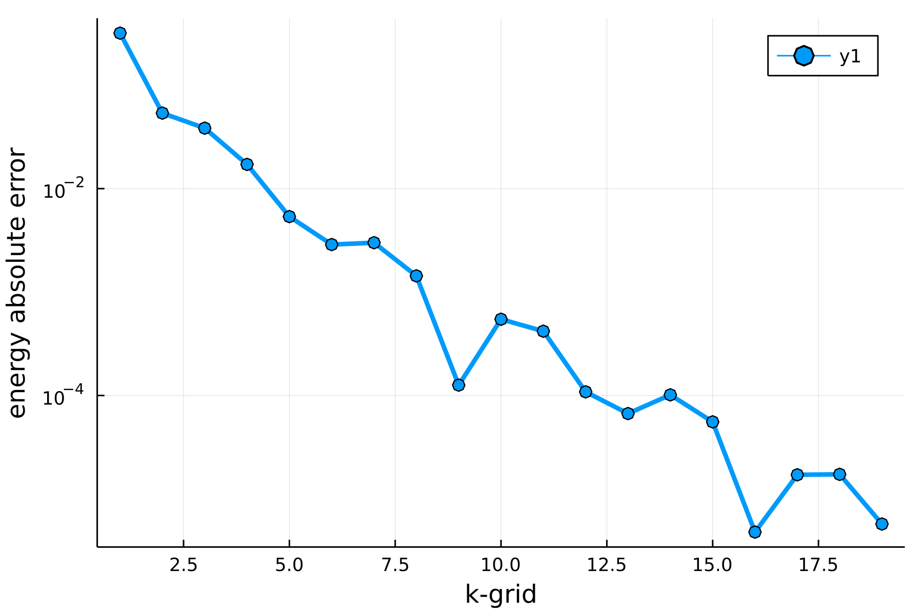
nkpt_conv = result.nkpt_conv5… and plot the obtained convergence:
using Plots
plot(result.nkpts, result.errors, dpi=300, lw=3, m=:o, yaxis=:log,
     xlabel="k-grid", ylabel="energy absolute error")
We continue to do the convergence in Ecut using the suggested $k$-point grid.
function converge_Ecut(Ecuts; nkpt, tol)
    energies = [run_scf(; nkpt, tol=tol/100, Ecut).energies.total for Ecut in Ecuts]
    errors = abs.(energies[1:end-1] .- energies[end])
    iconv = findfirst(errors .< tol)
    (; Ecuts=Ecuts[1:end-1], errors, Ecut_conv=Ecuts[iconv])
end
result = converge_Ecut(Ecuts; nkpt=nkpt_conv, tol)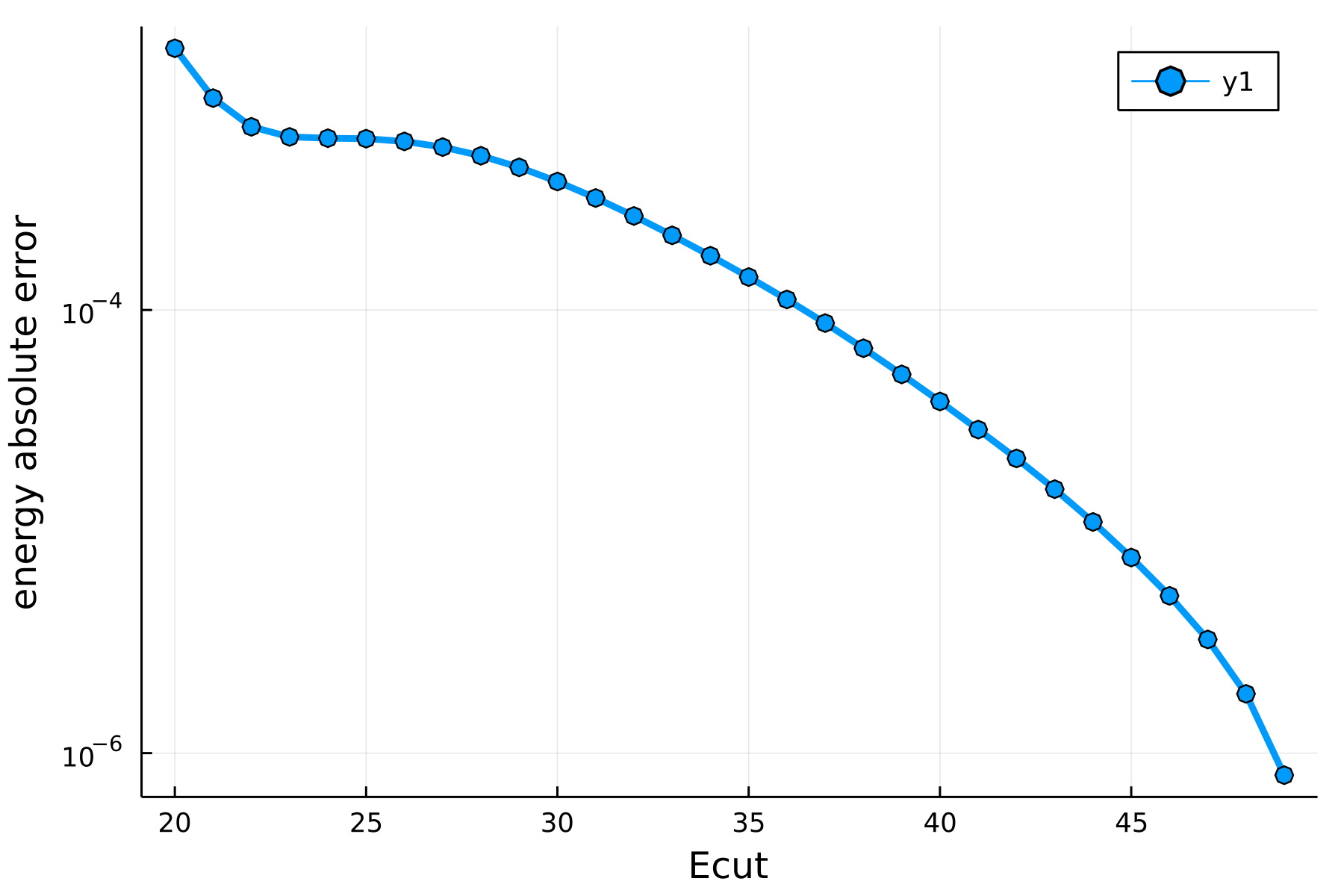
Ecut_conv = result.Ecut_conv18… and plot it:
plot(result.Ecuts, result.errors, dpi=300, lw=3, m=:o, yaxis=:log,
     xlabel="Ecut", ylabel="energy absolute error")
A more realistic example.
Repeating the above exercise for more realistic settings, namely …
tol   = 1e-4  # Tolerance to which we target to converge
nkpts = 1:20  # K-point range checked for convergence
Ecuts = 20:1:50;
…one obtains the following two plots for the convergence in kpoints and Ecut.