Timings and parallelization

This section summarizes the options DFTK offers to monitor and influence performance of the code. For details on running DFTK on HPC systems, see also Using DFTK on compute clusters and Using DFTK on GPUs.

Timing measurements

By default DFTK uses TimerOutputs.jl to record timings, memory allocations and the number of calls for selected routines inside the code. These numbers are accessible in the object DFTK.timer. Since the timings are automatically accumulated inside this datastructure, any timing measurement should first reset this timer before running the calculation of interest.

For example to measure the timing of an SCF:

DFTK.reset_timer!(DFTK.timer)
scfres = self_consistent_field(basis, tol=1e-5)

DFTK.timer

────────────────────────────────────────────────────────────────────────────────
                                       Time                    Allocations      
                              ───────────────────────   ────────────────────────
      Tot / % measured:            333ms /  46.9%           81.3MiB /  59.8%    

Section               ncalls     time    %tot     avg     alloc    %tot      avg
────────────────────────────────────────────────────────────────────────────────
self_consistent_field      1    156ms  100.0%   156ms   48.6MiB  100.0%  48.6MiB
  LOBPCG                  24   61.1ms   39.1%  2.55ms   11.9MiB   24.4%   506KiB
    DftHamiltonian...     66   52.4ms   33.5%   794μs   3.87MiB    8.0%  60.0KiB
      local              437   50.6ms   32.4%   116μs   88.8KiB    0.2%     208B
      nonlocal            66    731μs    0.5%  11.1μs    281KiB    0.6%  4.26KiB
    ortho! X vs Y         60   2.55ms    1.6%  42.5μs   1.47MiB    3.0%  25.1KiB
      ortho!             126   1.41ms    0.9%  11.2μs    805KiB    1.6%  6.39KiB
    rayleigh_ritz         42   2.45ms    1.6%  58.4μs   0.99MiB    2.0%  24.0KiB
    Update residuals      66    504μs    0.3%  7.63μs   0.99MiB    2.0%  15.4KiB
    ortho!                24    360μs    0.2%  15.0μs    121KiB    0.2%  5.03KiB
    preconditioning       66    239μs    0.2%  3.62μs   18.0KiB    0.0%     280B
  energy_hamiltonian       9   55.5ms   35.5%  6.17ms   13.7MiB   28.1%  1.52MiB
    ene_ops                9   54.1ms   34.6%  6.01ms   10.2MiB   21.0%  1.13MiB
      ene_ops: xc          9   52.0ms   33.2%  5.78ms   5.00MiB   10.3%   568KiB
      ene_ops: har...      9   1.44ms    0.9%   160μs   4.06MiB    8.4%   462KiB
      ene_ops: non...      9    210μs    0.1%  23.4μs    132KiB    0.3%  14.6KiB
      ene_ops: kin...      9    143μs    0.1%  15.9μs   86.3KiB    0.2%  9.59KiB
      ene_ops: local       9    110μs    0.1%  12.2μs    843KiB    1.7%  93.7KiB
  compute_density          8   26.7ms   17.1%  3.33ms   5.12MiB   10.5%   655KiB
    symmetrize_ρ           8   21.3ms   13.6%  2.66ms   3.96MiB    8.2%   507KiB
  energy                   8   8.35ms    5.3%  1.04ms   7.58MiB   15.6%   971KiB
    energy: xc             8   6.49ms    4.2%   812μs   2.95MiB    6.1%   378KiB
    ene_ops: hartree       8   1.21ms    0.8%   152μs   3.61MiB    7.4%   462KiB
    ene_ops: nonlocal      8    215μs    0.1%  26.8μs    132KiB    0.3%  16.5KiB
    ene_ops: kinetic       8    146μs    0.1%  18.2μs   78.1KiB    0.2%  9.77KiB
    ene_ops: local         8    124μs    0.1%  15.5μs    749KiB    1.5%  93.7KiB
  Anderson acceler...      7   1.64ms    1.0%   234μs   3.42MiB    7.0%   500KiB
  ortho_qr                 3    121μs    0.1%  40.4μs    101KiB    0.2%  33.7KiB
  χ0Mixing                 8   49.3μs    0.0%  6.16μs   33.8KiB    0.1%  4.22KiB
enforce_real!              1   57.2μs    0.0%  57.2μs      384B    0.0%     384B
────────────────────────────────────────────────────────────────────────────────

The output produced when printing or displaying the DFTK.timer now shows a nice table summarising total time and allocations as well as a breakdown over individual routines.

Rough timing estimates

A very (very) rough estimate of the time per SCF step (in seconds) can be obtained with the following function. The function assumes that FFTs are the limiting operation and that no parallelisation is employed.

function estimate_time_per_scf_step(basis::PlaneWaveBasis)
    # Super rough figure from various tests on cluster, laptops, ... on a 128^3 FFT grid.
    time_per_FFT_per_grid_point = 30 #= ms =# / 1000 / 128^3

    (time_per_FFT_per_grid_point
     * prod(basis.fft_size)
     * length(basis.kpoints)
     * div(basis.model.n_electrons, DFTK.filled_occupation(basis.model), RoundUp)
     * 8  # mean number of FFT steps per state per k-point per iteration
     )
end

"Time per SCF (s):  $(estimate_time_per_scf_step(basis))"

"Time per SCF (s):  0.008009033203124998"

Options for parallelization

At the moment DFTK offers two ways to parallelize a calculation, firstly shared-memory parallelism using threading and secondly multiprocessing using MPI (via the MPI.jl Julia interface). MPI-based parallelism is currently only over $k$-points, such that it cannot be used for calculations with only a single $k$-point. There is also support for Using DFTK on GPUs.

The scaling of both forms of parallelism for a number of test cases is demonstrated in the following figure. These values were obtained using DFTK version 0.1.17 and Julia 1.6 and the precise scalings will likely be different depending on architecture, DFTK or Julia version. The rough trends should, however, be similar.

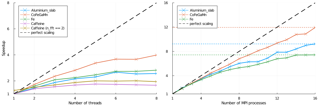
The MPI-based parallelization strategy clearly shows a superior scaling and should be preferred if available.

MPI-based parallelism

Currently DFTK uses MPI to distribute on $k$-points only. This implies that calculations with only a single $k$-point cannot use make use of this. For details on setting up and configuring MPI with Julia see the MPI.jl documentation.

1. First disable all threading inside DFTK, by adding the following to your script running the DFTK calculation:

   using DFTK
   disable_threading()

2. Run Julia in parallel using the mpiexecjl wrapper script from MPI.jl:

   mpiexecjl -np 16 julia myscript.jl

   In this -np 16 tells MPI to use 16 processes and -t 1 tells Julia to use one thread only. Notice that we use mpiexecjl to automatically select the mpiexec compatible with the MPI version used by MPI.jl.

As usual with MPI printing will be garbled. You can use

DFTK.mpi_master() || (redirect_stdout(); redirect_stderr())

at the top of your script to disable printing on all processes but one.

Thread-based parallelism

Threading in DFTK currently happens on multiple layers distributing the workload over different $k$-points, bands or within an FFT or BLAS call between threads. At its current stage our scaling for thread-based parallelism is worse compared MPI-based and therefore the parallelism described here should only be used if no other option exists. To use thread-based parallelism proceed as follows:

1. Ensure that threading is properly setup inside DFTK by adding to the script running the DFTK calculation:

   using DFTK
   setup_threading()

   This disables FFT threading and sets the number of BLAS threads to the number of Julia threads.

2. Run Julia passing the desired number of threads using the flag -t:

   julia -t 8 myscript.jl

For some cases (e.g. a single $k$-point, fewish bands and a large FFT grid) it can be advantageous to add threading inside the FFTs as well. One example is the Caffeine calculation in the above scaling plot. In order to do so just call setup_threading(n_fft=2), which will select two FFT threads. More than two FFT threads is rarely useful.

Advanced threading tweaks

The default threading setup done by setup_threading is to select one FFT thread, and use Threads.nthreads() to determine the number of DFTK and BLAS threads. This section provides some info in case you want to change these defaults.

BLAS threads

All BLAS calls in Julia go through a parallelized OpenBlas or MKL (with MKL.jl. Generally threading in BLAS calls is far from optimal and the default settings can be pretty bad. For example for CPUs with hyper threading enabled, the default number of threads seems to equal the number of virtual cores. Still, BLAS calls typically take second place in terms of the share of runtime they make up (between 10% and 20%). Of note many of these do not take place on matrices of the size of the full FFT grid, but rather only in a subspace (e.g. orthogonalization, Rayleigh-Ritz, ...) such that parallelization is either anyway disabled by the BLAS library or not very effective. To set the number of BLAS threads use

using LinearAlgebra
BLAS.set_num_threads(N)

where N is the number of threads you desire. To check the number of BLAS threads currently used, you can use BLAS.get_num_threads().

DFTK threads

On top of BLAS threading DFTK uses Julia threads in a couple of places to parallelize over $k$-points (density computation) or bands (Hamiltonian application). The number of threads used for these aspects is controlled by default by Threads.nthreads(), which can be set using the flag -t passed to Julia or the environment variable JULIA_NUM_THREADS. Optionally, you can use setup_threading(; n_DFTK) to set an upper bound to the number of threads used by DFTK, regardless of Threads.nthreads() (for instance, if you want to thread several DFTK runs and don't want DFTK's threading to interfere with that).

FFT threads

Since FFT threading is only used in DFTK inside the regions already parallelized by Julia threads, setting FFT threads to something larger than 1 is rarely useful if a sensible number of Julia threads has been chosen. Still, to explicitly set the FFT threads use

using FFTW
FFTW.set_num_threads(N)

where N is the number of threads you desire. By default no FFT threads are used, which is almost always the best choice.