Creating slabs with ASE

ASE is short for the atomistic simulation environment, a Python package to simplify the process of setting up, running and analysing results from atomistic simulations across different programs. Extremely powerful in this respect are the routines this code provides for setting up complicated systems (including surface-adsorption scenarios, defects, nanotubes, etc). See also the ASE installation instructions.

This example shows how to use ASE to setup a particular gallium arsenide surface and run the resulting calculation in DFTK. If you are less interested in having access to the full playground of options in DFTK, but more interested in performing analysis in ASE itself, have a look at asedftk. This package provides an ASE-compatible calculator class based on DFTK, such that one may write the usual Python scripts against ASE, but the calculations are still run in DFTK.

The particular example we consider the (1, 1, 0) GaAs surface separated by vacuum with the setup slightly adapted from ^[RCW2001].

Parameters of the calculation. Since this surface is far from easy to converge, we made the problem simpler by choosing a smaller Ecut and smaller values for n_GaAs and n_vacuum. More interesting settings are Ecut = 15 and n_GaAs = n_vacuum = 20.

miller = (1, 1, 0)   # Surface Miller indices
n_GaAs = 2           # Number of GaAs layers
n_vacuum = 4         # Number of vacuum layers
Ecut = 5             # Hartree
kgrid = (4, 4, 1);   # Monkhorst-Pack mesh

Use ASE to build the structure:

using PyCall

ase_build = pyimport("ase.build")
a = 5.6537  # GaAs lattice parameter in Ångström (because ASE uses Å as length unit)
gaas = ase_build.bulk("GaAs", "zincblende", a=a)
surface = ase_build.surface(gaas, miller, n_GaAs, 0, periodic=true);

Get the amount of vacuum in Ångström we need to add

d_vacuum = maximum(maximum, surface.cell) / n_GaAs * n_vacuum
surface = ase_build.surface(gaas, miller, n_GaAs, d_vacuum, periodic=true);

Write an image of the surface and embed it as a nice illustration:

pyimport("ase.io").write("surface.png", surface * (3, 3, 1),
                         rotation="-90x, 30y, -75z")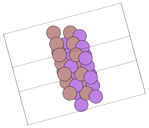

Use the load_atoms and load_lattice functions to convert to DFTK datastructures. These two functions not only support importing ASE atoms into DFTK, but a few more third-party datastructures as well. Typically the imported atoms use a bare Coulomb potential, such that appropriate pseudopotentials need to be attached in a post-step:

using DFTK

atoms = load_atoms(surface)
atoms = [ElementPsp(el.symbol, psp=load_psp(el.symbol, functional="pbe")) => position
         for (el, position) in atoms]
lattice = load_lattice(surface);

We model this surface with (quite large a) temperature of 0.01 Hartree to ease convergence. Try lowering the SCF convergence tolerance (tol) or the temperature or try mixing=KerkerMixing() to see the full challenge of this system.

model = model_DFT(lattice, atoms, [:gga_x_pbe, :gga_c_pbe],
                  temperature=0.001, smearing=DFTK.Smearing.Gaussian())
basis = PlaneWaveBasis(model; Ecut, kgrid)

scfres = self_consistent_field(basis, tol=1e-4, mixing=LdosMixing());

n     Free energy       Eₙ-Eₙ₋₁     ρout-ρin   α      Diag
---   ---------------   ---------   --------   ----   ----
  1   -16.61272253614         NaN   2.60e-01   0.80    4.8
  2   -16.73252199953   -1.20e-01   9.46e-02   0.80    1.0
  3   -16.73605366431   -3.53e-03   2.55e-02   0.80    3.5
  4   -16.73641744916   -3.64e-04   6.60e-03   0.80    2.2
  5   -16.73644314068   -2.57e-05   2.26e-03   0.80    3.0

scfres.energies

Energy breakdown (in Ha):
    Kinetic             5.8451470 
    AtomicLocal         -105.5844459
    AtomicNonlocal      2.3505291 
    Ewald               35.5044300
    PspCorrection       0.2016043 
    Hartree             49.5410298
    Xc                  -4.5946068
    Entropy             -0.0001307

    total               -16.736443140679